
This is the ultimate guide on Monte Carlo Analysis. With it, I have the ambitious goal of creating the only resource you need to learn about Monte Carlo analysis, find how to implement it in Excel, and understand all the statistics behind it. I don’t just want to show you what Monte Carlo is and how to use it, but I want to train your mind in a way that you can recognize any problem worth solving with Monte Carlo.
Like in the previous guide on Python in Excel, we have a lot to cover here. It does not matter if you don’t have any experience with Excel or Monte Carlo, this guide is from zero to hero and assumes no prior knowledge. Even if you are an expert, I structured it in sections so that you can go to the parts that interest you.
We have a lot of material to cover, so take a look at the table of content.
- What is Monte Carlo Analysis
- How to do a Monte Carlo Analysis in Excel
- Advanced Monte Carlo Analysis in Excel
- Conclusion
Let’s get started!
What is Monte Carlo Analysis
Monte Carlo Analysis in Brief
In this guide, I want to focus on making you understand what Monte Carlo analysis really is. More true knowledge, less formal definitions. So, if I have to give my own definition I would say:
Monte Carlo Analysis is a way to predict the future based on statistical probability.
Rather than predicting an exact future, however, you want to predict the most likely scenario. This prediction, or forecasting to use a more business-friendly term, is based on random values. At this point, people get scary: how can a forecast be accurate if it is based on random values? Thanks to statistics, it can, and we will explain why.
The Monte Carlo analysis (or method, or model) takes its name from Monte Carlo, the casino town in the French Riviera (note that the city is not in France, but in a separate tiny state). Just like in our analysis, in a casino there is some randomness about whether you are going to win or not. However, it is not pure random: there are some probabilities behind it.

Let’s imagine a simple bet: flipping a coin. You know you have a 50% chance of getting a head, and 50% chance of getting a tail for every flip you do. If you have to predict what will happen in the next flip, you know you will get 1 head (or 1 tail, for the matter), but you can only be 50% confident that your forecast will happen.
In this game, if you win you get 1$ and if you lose you lose 1$. You start with 5$, and you want to know after how many flips you will stop playing. You can’t know for sure unless you play, because there is some randomness (you don’t know exactly what you are going to get, if head or tail). With a Monte Carlo Analysis, you can forecast how many games you can play.
In my Monte Carlo Analysis, if I start with 5$ I can expect to stop playing after 95 flips on average. Sometimes I will be able to play much more, sometimes much less, but on average I can expect to do 95 flips before running out of money. If I start with a 2$ budget, however, I can expect only 44 flips on average before I go bankrupt.
We can use the Monte Carlo Analysis to forecast scenarios like this, using a mix of random variables based on probability (like the coin flip) and known values. For example, we can use Monte Carlo Analysis to evaluate the value of acquiring a company, estimating the cost savings from merging the two companies together with probability but knowing for a fact the legal fees for the merger.
How does the Monte Carlo Analysis Work
At this point, we know that a Monte Carlo Analysis uses some probability and some known values to forecast something in the future. But how does it work exactly? Performing a Monte Carlo Analysis in Excel is a series of steps you can perform sequentially:
- Define your problem as a set of variables and formulas around those variables. Put some static values in your input variables to verify your model makes sense.
- Replace input variables with random values generated out of a probability distribution.
- Have Excel run the problems for many different combinations of input variables and log all the results.
- On the list of results, extrapolate the most common range (e.g., 90% of results fall between X and Y).
We will see the details of each step in a bit, including how to practically do it in Excel. However, for this section, we can use an example to make things clearer: imagine you have to compute the payment you need to do for a mortgage you still need to take.
The payment of a mortgage is mainly influenced by 3 items: the duration of the mortgage, the principal (the amount you borrow), and the interest rate. You already know that you want a 20 years mortgage, that is a given. However, you are still unsure how much you will borrow and what is the interest rate you will have. You can use a Monte Carlo analysis to estimate it.
With the Monte Carlo analysis, you generate random interest rates and principal amounts, use them together to compute the payment (with the =PMT function in Excel) and store the results. Then, when you ran this model for 1000 times (or any other number of times you like), you take stock on the results and see what will be the most common range of payments.
Now, remember that with Monte Carlo analysis variables are NOT completely random. In fact, they follow a probability distribution. A probability distribution is a statistical tool that allows you to generate random but likely values. There are various types of distribution, but the most common we use is the standard distribution. With that, we have a central value that is the most common, and a range around that value. Values close to the center value are more common, and the further you get away from that, the less probable a value is.
For example, if your principal il $200k with a range of plus/minus $20k it will be much more common to get values around $200k than at $190k, and extremely unlikely (but still possible) to get a value of $150k or $250k.
But each single combination is of little value by itself. To have some meaningful result, we need to follow the rule of large numbers. That is, we need to run as many combinations as possible and see what output they produce. Most of the times, we will get a likely interest rate with a likely principal, and only extremely rarely we will get an uncommon interest rate and an out-of-ordinary principal. Sometimes we will get an interest rate above average, sometimes below average, and they will tend to cancel out with each other.
All of this means that we can have of a set of results and we can find the mean, the standard deviation (how far they tend to part away from the mean), and what is the range where 90% of results are. This gives us much more confidence instead of having a static number as a forecast. Note that to run the model many times and produce the output, we will need to rely on Visual Basic for Application (VBA).
We will explain how to do everything technically as part of this guide to the Monte Carlo Analysis. So, even if you have no clue how to do all this in Excel, we will go through it step by step here. Before we do this, however, it is important to understand why we do this: why is the Monte Carlo Analysis a superior forecasting method?
Advantages of Monte Carlo Approach
We know now that the Monte Carlo Analysis is an approach to forecasting. There are so many possible ways to create a forecast, so why is Monte Carlo superior?
- It produces a forecast with an explicit measure of precision/uncertainty
Instead of saying “the result will be X”, we say “the result will be between X and Y in W% of cases”. If we forecast just a number, we have no idea of the precision of the forecast. Monte Carlo solves this problem, presenting each estimate with a confidence interval. - You can mix variables with different level of confidence
We know the outcome is a confidence interval value, but also input variables can (and should) be defined in the same way. You can create a Monte Carlo analysis that is based on some unknown variables, defined from a probability distribution, and some certain variables defined as a static number. This gives you a lot of flexibility in what you can accomplish. - It runs in Excel
This may be obvious, but it is a great advantage. There are other forecasting techniques that may yield more precise results, for example artificial intelligence. However, they require dedicated software, often extremely powerful hardware, and they are hard to implement. Instead, you can create a Monte Carlo Analysis in Excel in even 5 minutes (note: complex problems will require more time, of course). - You can forecast everything
See point 1. Since the Monte Carlo Analysis comes with a measure of precision, you can forecast literally anything. Some forecasts, where you have more data, will come with a higher degree of precision, while others will come with low precision (and thus, high uncertainty: their interval will be wide and their confidence will be low).
I hope those advantages convince you that Monte Carlo Analysis is a tool you need to have under your belt. If not, you can take a look at where this method is used and think if you see yourself in those roles.
Where is Monte Carlo Analysis used?
Or rather, who uses monte Carlo Analysis? Pretty much anyone that is serious about forecasting something happening in the future. It is particularly used in the financial industry and to make management decisions. The two are often interlinked.
The classic example in the financial industry is predicting the price of a stock. We can do this based on historical data (we will do this in the Advanced section of this guide), or we may use other parameters such as sales, costs, and even weather forecasts (e.g., a hotter summer may result in more sales for an ice-cream brand).
But the most common usage of Monte Carlo analysis is for decision-making. You need to make a decision that will result in something uncertain in the future, how do you ensure you make the best decisions that maximize your odds? Monte Carlo analysis will help you here. This is often used in business: should we buy this product from a supplier, or buy it ourselves? Should we rent the office, or buy it? Should we acquire this other company, or license their brand? All of these decisions and more can be modeled with Monte Carlo. In fact, any decision can.
But this decision-making doesn’t have to be business related. You can use Monte Carlo for personal decision-making. Whenever you have a big decision to make, you can use Monte Carlo to help you out. For example, I have recently used this process to evaluate the possibility to purchase a house, considering the odds of myself relocating in the next few years, the cost of rent, the transaction costs of buying/selling, and more parameters.
To sum it all up, in business you will find a bunch of people running Monte Carlo Analysis, or at least using their results: data scientists, managers, chief executives, financial analysts, bankers, insurance agents. If you see yourself in any of those roles, then you need to learn how to do a Monte Carlo analysis. And even if you don’t see yourself there, this is a tool anyone should know to make better decisions.
How to do a Monte Carlo Analysis in Excel
Quick Guide to Monte Carlo Analysis
In this section we will see how to create a Monte Carlo analysis quickly and end-to-end. In later sections we will explore all the different aspects of it and provide explanations. But, if you are in a rush, look here and you will be able to create your own analysis.
First, define a problem you want to solve and create a spreadsheet to do that. Ideally, this is done by having a set of variables and some other cells where you have some formulas that calculate the results. Whenever you input different values in your input variables, you will get different results.
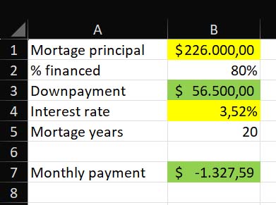
In our case, we have a simple problem where we have two variables as input (in yellow) and two variables as output (in green).
Instead of inputting values manually in the yellow cells, use NORM.INV to generate a random value starting from a mean (central value around which we generate random values) and a standard deviation, that is, how likely it is that values may be far away from the mean. For example, we use the following two formulas respectively for principal and for interest rate.
=ROUND(NORM.INV(RAND();200;20);0)*1000=NORM.INV(RAND();0,034;0,005)Then, create another sheet named “MC” with a table named “montecarlo”, one column named trial and one column for each output variable you want to store (downpayment and monthly payment). Create this table by leaving the first 6 rows empty (start the table at A6). Put a reference to your output formulas in B1 that points to the cell containing the downpayment, and in C1 to the cell containing the monthly payment.
For example, since downpayment was in B3 in “Sheet1”, use the following formula in B1 of “MC” sheet.
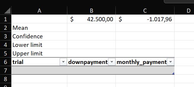
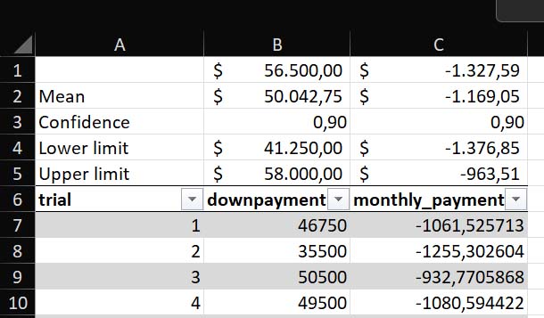
=Sheet1!B3The space that we left before the table is for some items we will compute for each column: mean, confidence, lower and upper limit. The result should look like this.
Now, open the VBA editor, copy the following Macro in a new module and run it.
Sub MonteCarloMacro()
    Dim ws As Worksheet
    Dim tbl As ListObject
    Dim i As Long

    ' Set the worksheet where you want to insert the data
    Set ws = ThisWorkbook.Worksheets("MC") ' Change "MC" to your sheet's name

    ' Set the table
    On Error Resume Next
    Set tbl = ws.ListObjects("montecarlo")
    On Error GoTo 0

    ' Initialize iteration number
    i = 1

    ' Loop 1000 times and add data to the table
    For i = 1 To 1000
        ' Add the data to the table
        tbl.ListRows.Add AlwaysInsert:=True
        tbl.ListRows(i).Range.Cells(1, 1).Value = i
        tbl.ListRows(i).Range.Cells(1, 2).Value = ws.Cells(1, 2).Value ' B1
        tbl.ListRows(i).Range.Cells(1, 3).Value = ws.Cells(1, 3).Value ' C1
    Next i
End Sub
Finally, use cells B2 through B5 and C2 through C5 to compute mean the mean, lower and upper limit. Here are the formulas you should have in. You can find also the text values for easy copy-paste (European Excel version).
=AVERAGE(montecarlo3[downpayment])=PERCENTILE.INC(montecarlo3[downpayment];(1-B3)/2)=PERCENTILE.INC(montecarlo3[downpayment];1-(1-B3)/2)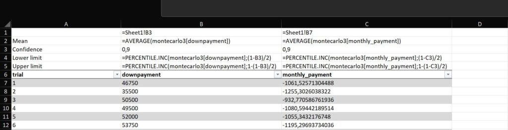
There we go, you now have the most common range for downpayment and monthly payment. You can be 90% confident that your downpayment will be in this range, and so will your monthly payment. If this is too quick, let’s go over the various steps one by one.
Create a Monte Carlo Analysis Model
The first step is to define the problem you want to solve. I recommend doing it with a series of parameters and formulas: you write the name of the parameter in the first column, and the value you want for it in the second column. For more complex problems, you can use tables and other data structures, but for this quick example let’s keep things simple.
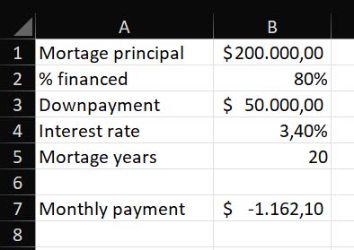
In this example, we want to compute the monthly payment of a mortgage we are thinking about getting. Let’s start by defining a spreadsheet that calculates the rate if we input data manually. Here are the formulas and values used in this example:
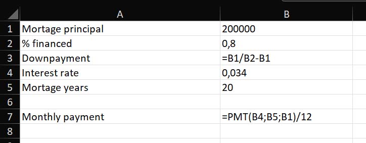
If we disable the “Show Formula” option, this is the result we have. With a principal of 200k, a rate of 3.4% and a duration of 20 years, we will need to pay 1162$ (note that in the picture I am using European numbers with dot to separate thousands).
Use NORM.INV and RAND to generate possible inputs
This problem works, but now we need to add some uncertainty. We are unsure how the rate will change over time, and we are not sure about the principal because we have not selected the house yet. We can use =NORM.INV and =RAND to generate a random value out of a standard distribution. =RAND will generate a random value between 0 and 1 every time the spreadsheet refreshes. =NORM.INV, instead, will produce a value out of a probability distribution, given a probability number.
We can use NORM.INV providing a random probability number with RAND, a center value and a standard deviation. The center value is the most common value, while the standard deviation indicates how “flat” the bell is. The less the standard deviation, the more the probability of generating values is concentrated around the center value. The larger the standard deviation, the more probable to get values further away from the center (but still, proportionally, a value closer to the center is still more likely than one far from the center).
This example generates a random value out of a standard distribution centered around the number 200 and with a standard deviation of 20. Note: I am using European formulas, replace semicolon with comma if you are using American Excel.
=NORM.INV(RAND();200;20)We want to use this and round it, so we get only integers roughly between 180 and 220, with numbers around 220 being more common. Then, we multiply this by 1000 to get the thousands amount of the principal. We could have created a distribution around 200k with a deviation of 20k, but then we would have generated many different values with decimal places. Instead, this allows us to show only 1k increments.
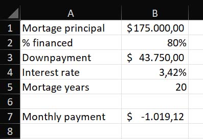
=ROUND(NORM.INV(RAND();200;20);0)*1000We can do something similar for the rate: we know the center range is 3.4%, but we know it can roughly vary of 0.5%.
=NORM.INV(RAND();0,034;0,005)Once again, we will get most values close to 3.4% (that is, 0.034 numeric value).
Now, you will see very time you change any value in any cell, Excell will re-compute principal and interest rate because RAND() will give a different value. However, looking at every new output generated manually is inconvenient. What we want to do now is run the model thousands of times and get the most likely results.
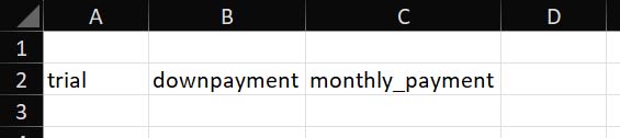
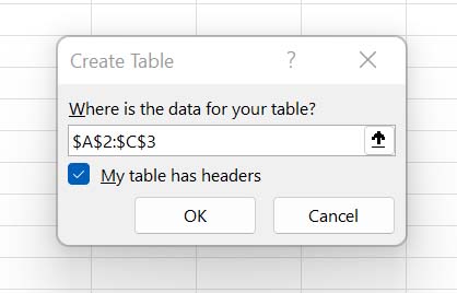
First, we need to create a table to store the Monte Carlo analysis’s results. Let’s create a new sheet, which we name “MC”, and in it a table starting from cell A2 (leave A1 blank, we will see later why). This table should contain 1 column to keep the trial number, and one column for each value we want to store out of the analysis. In this case, we will store two: downpayment, and monthly payment.
Then, select these three cells and the (empty) cells below them to create a table out of them.
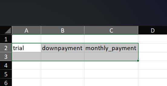
Now, with this range selected, go in Home > Format as a table. Select any layout you like when prompted.
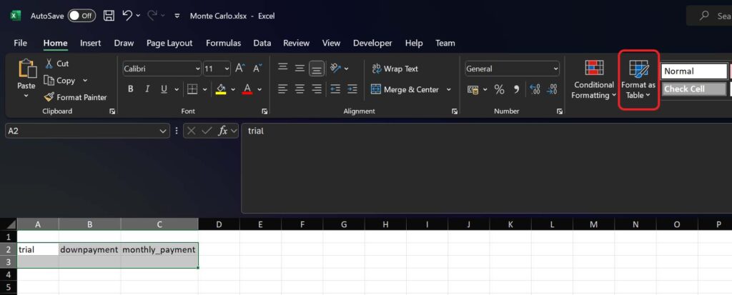
Select that your table has headers, since the fields that we just filled are the headers of the columns in the table.
Now, in the Table Design section, rename the table to “montecarlo”. You can use any name you like, but for our exercises we will use this name to make it clear what it is about. This table will store all the results for all the runs of our model.
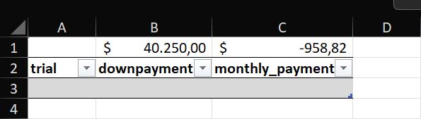
Now that we have a table ready, we need to create a reference to the output of the model, the values we want to store in our table every time we do an additional run. We simply add a reference to the cell that contains the output from our first sheet in the cells we left blank above the table.
We leave cell A1 blank, because that will not be about an output but just about the trial run. Then, we write the following code in cell B1 to reference the original cell containing the downpayment.
=Sheet1!B3And we add the following code in cell C1 to reference the cell of the monthly payment.
=Sheet1!B7Whenever downpayment or monthly payment change, they will reflect in the MC sheet immediately. Adding some nice formatting, this is the outcome we are looking for:
Write a Macro to compute the result multiple times
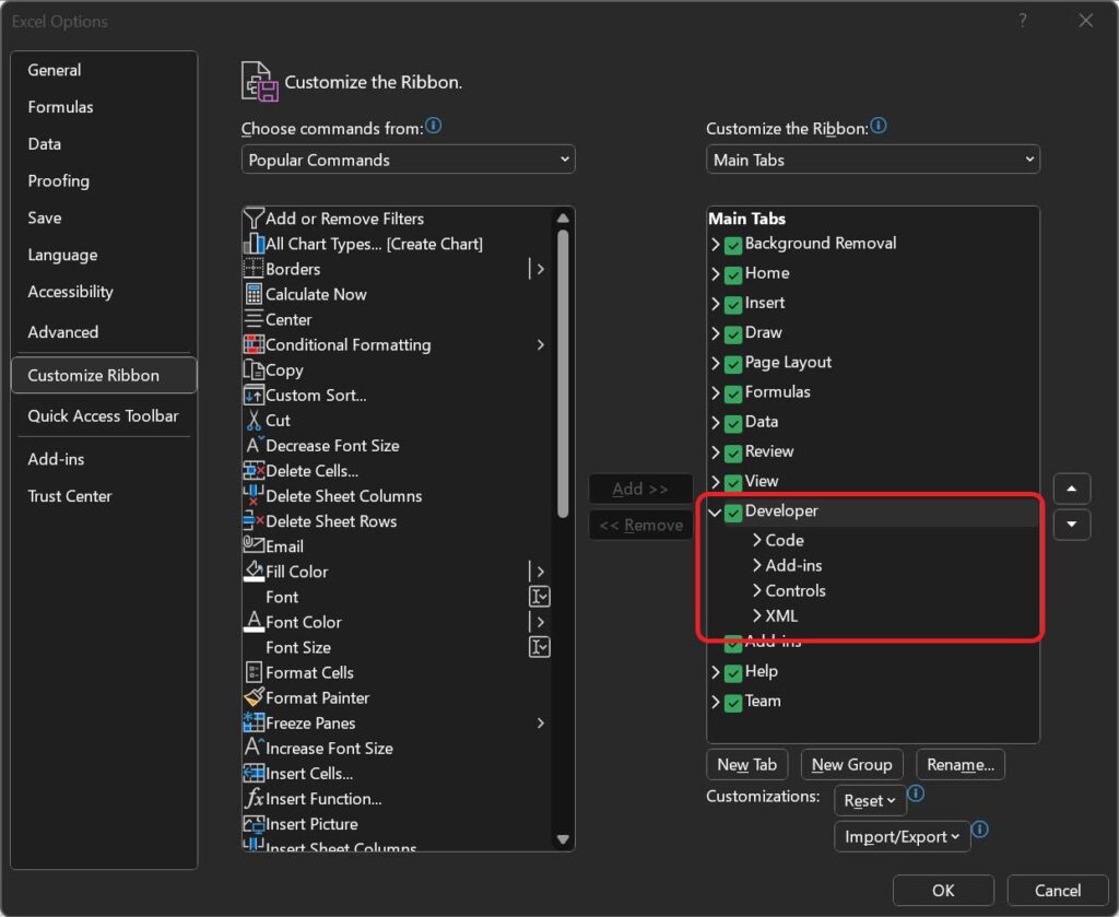
The next step is to create the VBA code that will fill this table. For this, you need Developer tools enabled, and have a Developer tab on top. In case you don’t have it, go to File > Options > Customize Ribbon and be sure that “Developer” is selected.
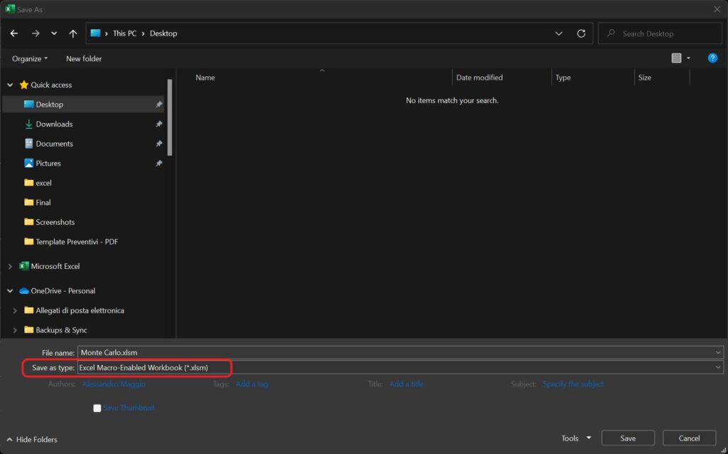
Now, Save your file as XLSM. This will ensure Macros are enabled. Do it now: you can create Macros even if you don’t save it as XLSM and they will run just fine. However, they won’t be stored and you won’t get any error, and when you re-open the file you realize they are not there anymore, losing a lot of progress. Go in File > Save As and select the Macro-enabled format.
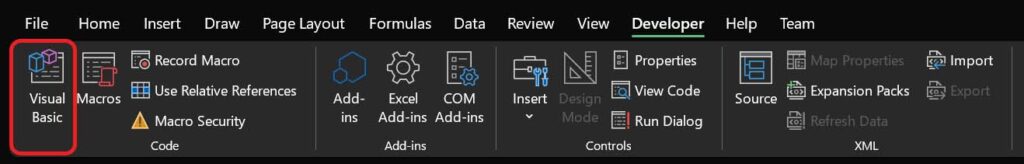
Finally, we can go in Developer tab and click Visual Basic to open the Visual Basic editor.
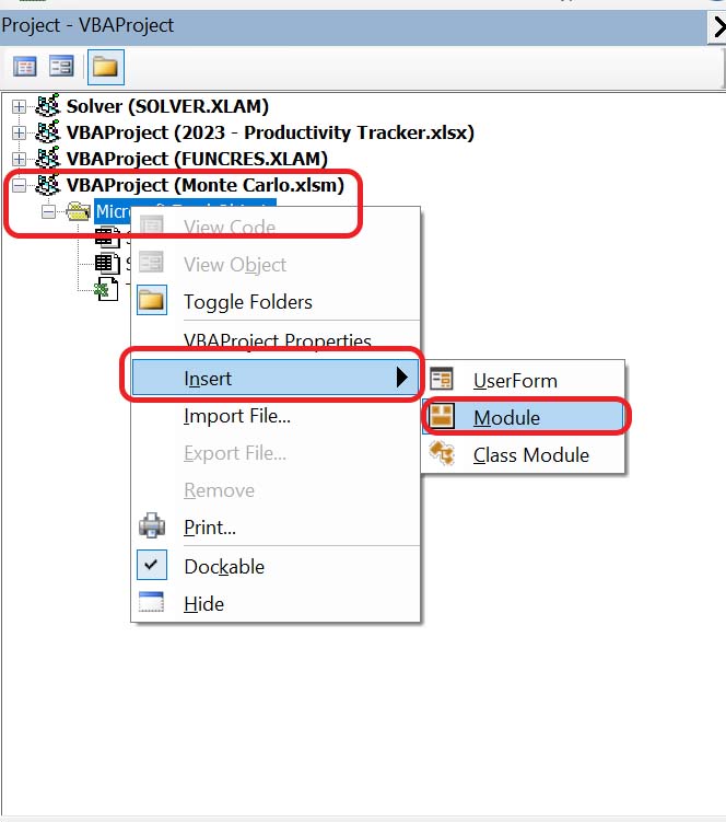
Once you have the editor open, you will see a list of VBA projects on the left side. Select Microsoft Excel Objects under the Excel file you are working on (for us, it is “Monte Carlo.xlsm”), and insert a new module by right clicking.
This will open the module on the right part of the screen (optionally, you can rename the module by editing the module name on the bottom-left box, this is not required and by default it is named “Module1”). The VBA editor is just a text editor, much like Notepad, where you can write VBA code. Paste the following code, which is already tested to work in our case-
Sub MonteCarloMacro()
    Dim ws As Worksheet
    Dim tbl As ListObject
    Dim i As Long

    ' Set the worksheet where you want to insert the data
    Set ws = ThisWorkbook.Worksheets("MC") ' Change "MC" to your sheet's name

    ' Set the table
    On Error Resume Next
    Set tbl = ws.ListObjects("montecarlo")
    On Error GoTo 0

    ' Initialize iteration number
    i = 1

    ' Loop 1000 times and add data to the table
    For i = 1 To 1000
        ' Add the data to the table
        tbl.ListRows.Add AlwaysInsert:=True
        tbl.ListRows(i).Range.Cells(1, 1).Value = i
        tbl.ListRows(i).Range.Cells(1, 2).Value = ws.Cells(1, 2).Value ' B1
        tbl.ListRows(i).Range.Cells(1, 3).Value = ws.Cells(1, 3).Value ' C1
    Next i
End Sub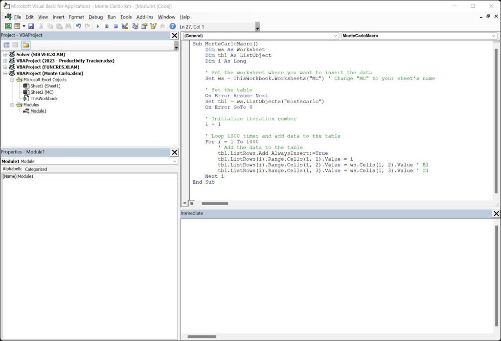
All you need to do now is to run the Macro, using the “play” button on the top of the VBA editor.
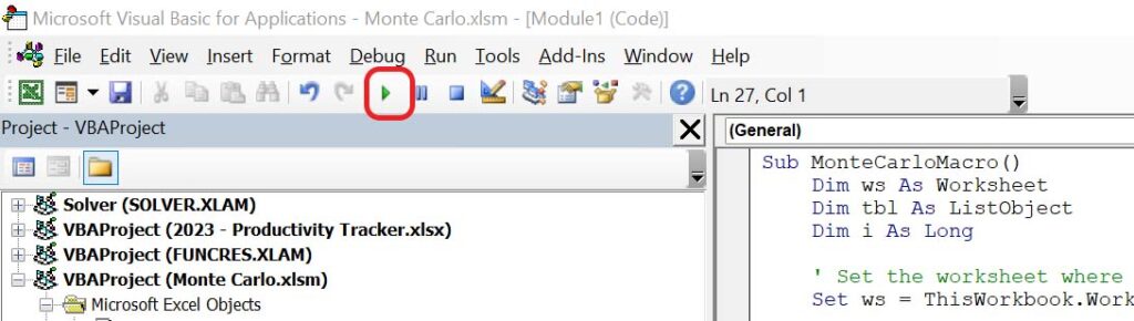
Running the macro will take a while, typically a few minutes depending on how powerful your computer is. What this macro does is take the values in cells B1 and C1 and copy them as new rows in our table. The final result will look something like this (your values will be different, as they are generated randomly every time):
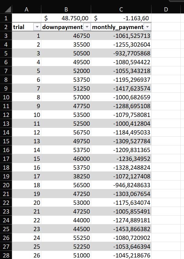
Results go all the way down to row 1001 (1000 results plus the header). In case you have an empty blank like as first item, you can simply delete it. This is because our macro starts to add data at the end of the table, so if you want to re-run the macro you should delete what’s already in the table first.
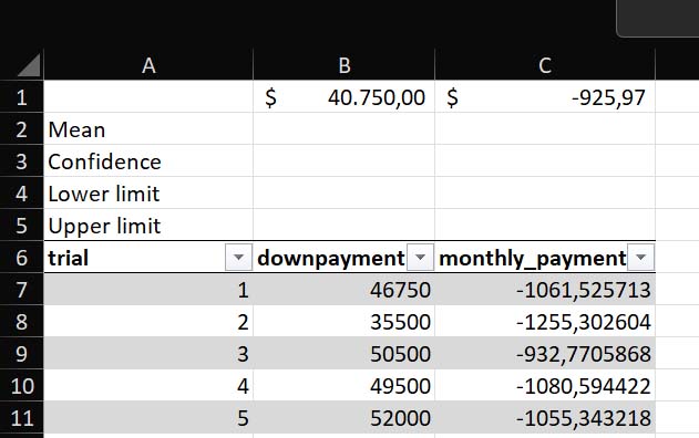
Find the confidence interval
Now, all it’s left to do is the analysis to figure out what are the most common values, our range for downpayment and for monthly payment. We will do this by calculating two percentile values. Let’s start by creating some cells by adding some new rows at the beginning of the table. In this way, we will compute mean, confidence, lower and upper limit for each column of the table (downpayment, monthly payment).
Computing the mean is simple, we can just use the AVERAGE function and select the entire range we want to use. For example, we will use the following formula in cell B2.
=AVERAGE(montecarlo[downpayment])Confidence, instead, is a value we choose. In this example, we want a confidence of 90%, that is, we want to find the range of values that contains 90% of the values generated by the model. Thus, 10% of the values will be outside of this range: 5% will be below it, and 5% will be above it. Let’s simply write 0.90 in the cell.
Now, we need to compute the lower limit. For that, we use the percentile function (explained in details later in the guide). If we want a confidence of 0.90, it means the lower limit is going to be 5th percentile (the 5% of values below the range). To compute that, we subtract our confidence interval from 1 (to get 0.10) and divide it by two. In other words, starting from 0.90, the following formula returns 0.05 (with confidence interval in cell B3).
=(1-B3)/2However, we do not want to write this formula. We want to use it to extract that percentile from the range, so let’s write the following code in cell B4.
=PERCENTILE.INC(montecarlo[downpayment];(1-B3)/2)The same logic applies to find the upper limit. However, in that case we want the 95% percentile. (90% starting from 5% = 95%). We do that simply by subtracting the 5% from 1, and thus use the following formula.
=PERCENTILE.INC(montecarlo[downpayment];1-(1-B3)/2)Here are the results.
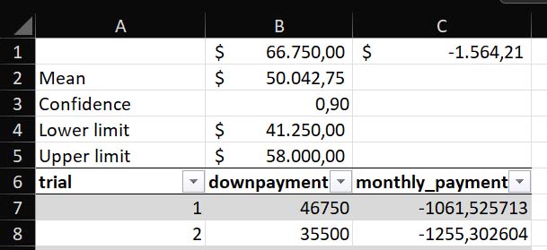
We can repeat the same process for the monthly payment, and thus get the following final result.
Advanced Monte Carlo Analysis
Statistics 101: Standard Deviation
If you want to be an expert on Monte Carlo Analysis in Excel (or even outside Excel), you need to know at least the basics of statistics. Specifically, you need to know standard deviation. To put it simply, standard deviation is a measure of how much your dataset is dispersed.
If you roll two dice, you will get a random number between 2 and 12. However, if you roll them over and over, you will see that more often than not you will get 7. That is because it is the most likely: there are 32 possible combinations, but 6 of them always generate 7 (1+6, 2+5, 3+4, 4+3, 5+2, 6+1). That’s more than any other possible result.
The same is true for any random value that is generated within some parameters: actual value will be random, but it will cluster around a mean. Standard deviation expresses how the dataset is clustered around the mean, or not.
The first step to compute standard deviation is to compute the mean in fact, the average of all datapoints. Then, for each datapoint we need to consider how far it is from the mean. We do that simply by subtracting the value of the mean from the datapoint. For example, if we have three numbers: 2, 5, and 8 the mean will be 5. The first number (2) is distant -3 from the mean (2-5 = -3), the second number 0, and the last number 3.
The problem with this, as we saw, is that distance from the mean can be negative if a number is below the mean. Since standard deviation is an expression of dispersion, we don’t care about direction, so we should square that distance, getting thus 18 (-3^2 + 0^2 + 3^2).
We then divide the value we obtain in this way by the number of items in our dataset, in our case, 3.We do this if our dataset represents the entire population, all items (that is, all possible items have been sampled, it is not like a survey where we pick random people because we cannot ask everyone). If we have only a sample, that is, some people or items are left behind and are not in our dataset, we divide by the entire population minus 1.
Let’s assume we have the entire population, we divide 18 by 3 and get 6. That is the variance, it expresses dispersion but it is not in the same scale of our dataset, because we have squared datapoints. To get back to the standard deviation, we need to do the square root of this. We get 2.45.
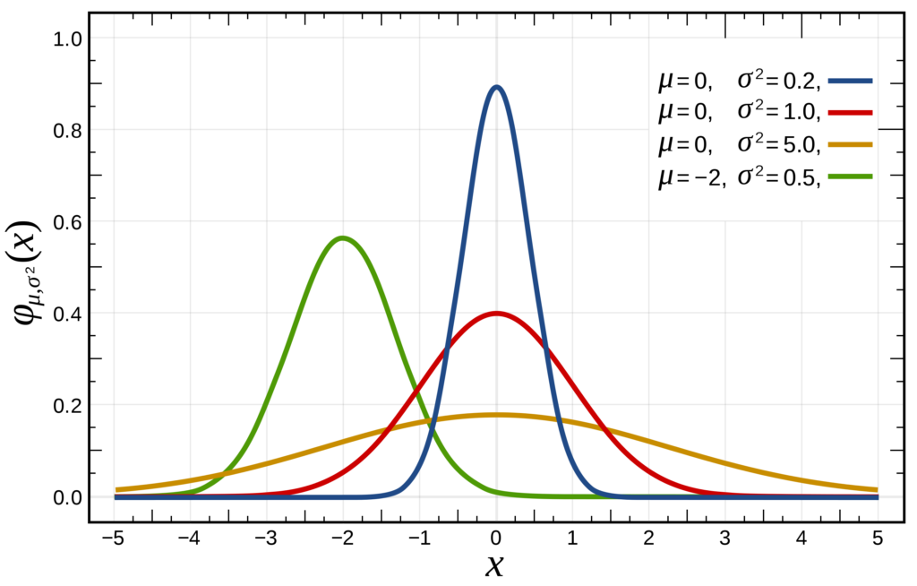
If we have a mean and we have a standard deviation, we can use it to generate random values. In a graph, the mean indicates where the bell curve peaks, the standard deviation indicates how flat or steep the bell is.
All this translates into a simple concept: with only two numbers (mean and standard deviation), we can generate realistic random values. The hard part is often identifying the right mean and the right standard deviation, but you know even just by intuition the value “around which” something stands.
Forecasting on historical data using standard deviation
One of the benefit of a normal distribution, that we compute with mean and standard deviation, is that we don’t need to estimate the mean and the deviation all the times. If we have historical data, we can simply use that to compute both mean (average of all dataset) and standard deviation (STDEV.S formula in Excel).
Let’s see how to do it in an example, on how to forecast stock prices. We start by having the price for a stock over a past period, say the past year. The stock price is measured daily, so we can subtract previous day’s from current day’s value to identify how much the stock went up or down on any given day. We can call this additional value “movement”. Then, we compute average and standard deviation on the movement, and not on the price.
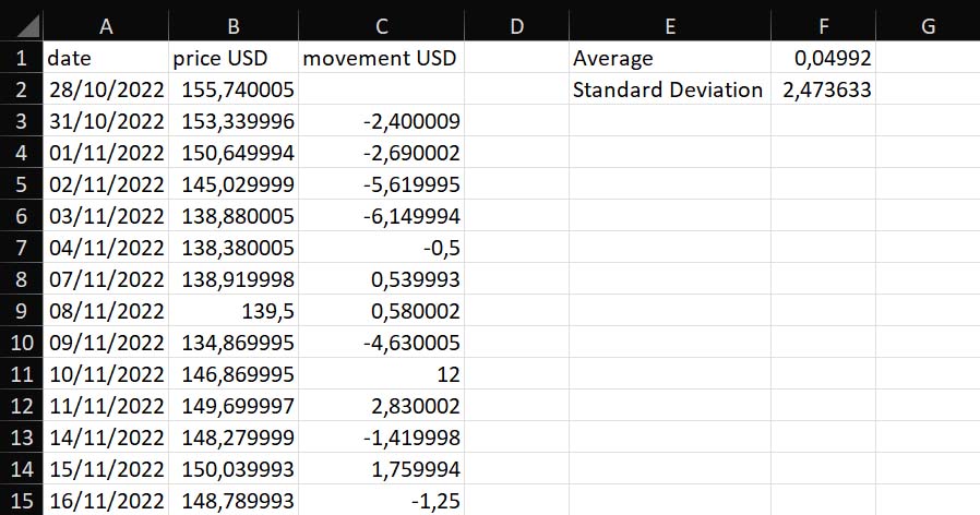
In cell F1, we have the following formula:
=AVERAGE(C3:C252)In cell F2, we have this instead:
=STDEV.S(C3:C252)Of course, the range C3:C252 contains all the movements. To compute movement, we simply have the formula that takes the price on the same line and subtracts the price of the previous line from it. Obviously, we start in the second cell since the first one has no previous. In C3, which is the first movement cell, we wrote:
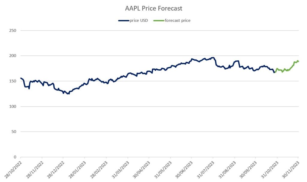
=B3-B2This is what our file looks like at this point. We are using Apple (AAPL) stock prices for 1 year ending on October 27, 2023.
At this point, we can go at the end of the dataset and add more lines, say for 1 more month, for our forecast. We then use the following formula to predict the movement (F1 and F2 are the cells that contain mean and standard deviation, respectively).
=NORM.INV(RAND();$F$1;$F$2)Here, we simply plot the movement right below the movement we calculate for historical data. Then, however, we want to have our forecast price in a separate new column, so that it will look nicer on our chart. For the first forecast price, we sum the movement we forecasted to the last price in the dataset. This goes in D253:
=B252+C253For any subsequent point, we sum the previous datapoint (which is a forecast by itself) with the movement forecasted for that point. This goes in D254:
=D253+C254If we plot all this, it will look something like this chart. Note that by adding the forecast in a separate column we can plot it with a different color on the chart.
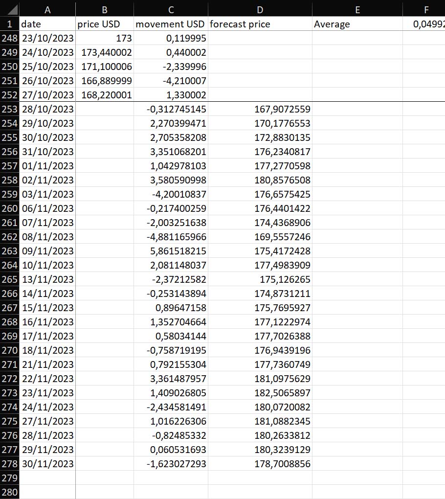
Of course, this is just one rand, and almost certainly the stock price will not evolve exactly like this. But we run this with a Montecarlo Model, using a Macro that performs 1000 attempts and storing the resulting price on the final day, then we can do an average and get a 90% confidence interval on what is a likely price one month from now.
Percentiles
In all this Montecarlo Analysis in Excel, we used percentiles to compute the confidence interval: the most likely range for the value we want to forecast. But what is a percentile exactly? In this section, we provide just a little bit of theory you need to understand percentiles.
A percentile is a number that you use to represent a dataset. Often, people use the mean (or average) to represent a dataset. This is intuitive: you have a bunch of datapoints, you sum all their values, divide that by how many datapoints you have, and you have the mean. In this way, you can find that the average age in Brazil is 33 years, or that a woman in Denmark will have 1.7 children in her life. The problem with this approach is that averages are not real. You can’t have 1.7 children, you either have 1 or 2. The mean is an artificial construct and does not represent any individual datapoint.
Means and averages can work well in some cases, but in our case, where we try to find the confidence interval, they are simply useless. Percentiles are different.
In a mean, you simply sum all the values and then divide by the number, you don’t care the order in which values are in. In percentiles, you care about the order. In fact, the first step is to rank all your dataset from smallest to largest. If you have the list of people living in Brazil and you are interested in age, you will rank them from the youngest to the oldest.
You will start with the people born today, and after them the people born tomorrow, and then somewhere down the road people born 10 years ago, and so on. If you want to be precise, you should rank them according to hour and minute in which they were born, even the day will not be granular enough. Of course, in Brazil you have millions of people, but for sake of simplicity imagine you have just 100.
Getting the 20 percentile it means you count 20 people, you stop on the 20th and check the age of that person. In this way, you know that 19 people are younger (because they were ordered) and 80 people are older. If instead of 100 datapoints you had 1000, then you would need to stop to the person number 200 (because 200 = 20% of 1000). If you had one million, on person number 200k, and so on.
The dataset does not need to grow linearly either, it can have steps. For example, if we take the children per woman in Danmark, we will have a lot of datapoints of all the same value of the beginning: 0. Then, at some specific percentile, we will jump at 1 and stay there for a while. After more datapoints we will reach 2, and the same for 3, 4 and so on. If the first woman who has at least one child is at percentile 25 (written as P25), it means if we get P0 (the smallest value) or P24 we will always get the value of 0, and only from P25 the value of 1.
We use percentiles mainly to discard outliers. For example, if we want to consider the net worth of people, there will be just a bunch of individuals that have extremely high net worth (Jeff Bezos, Elon Musk, Warren Buffet etc.) that alone can skew the statistics. If we want to consider net worth excluding those extra-rare cases, we could simply look at P95 to exclude the top 5%.
In our specific case, we use a low percentile (typically P5) and a high percentile (typically P95) to find a range where 90% of values reside.
Using different probability distributions
So far, we saw only the standard distribution in our Monte Carlo Analysis. That is the bell-shaped figure where the center of the bell is defined by the mean, and the steepness of it by the standard deviation. While this is by far the most common distribution, and the one that represents reality the best, it is not the only one.
Depending on circumstances, we may want to use other distributions. After all, a distribution in a Monte Carlo Analysis is a function, a rule that defines how to generate random values. We have several options, but the other common one that can be used is the uniform distribution.
In the uniform distribution, all values are equally likely to occur. They do not cluster around a center, the first value at the extreme left is as likely as the one at the extreme right, or at the center. As a consequence, this distribution looks like a flat line. We can use this when there is really no pattern and no clustering around something, and an event is purely random.
To plot this as a continuous uniform distribution (the technical name for it), we find a min and max value and then draw a line. To the left and right of this line, there is literally no possibility that a value will be generated.

In Excel, we achieve this with the RANDBETWEEN formula. For example, a uniform distribution between 0 and 10 will look something like:
=RANDBETWEEN(0, 10).This does integer increments. If we want to have continuous increments, we need to use RAND() that generates a random decimal value between 0 and 1, and multiply that for the maximum value of the range.
=RAND()*10If our distribution does not start at 0, say it is between 10 and 15, we then need to add the minimum (10) to the random value generated multiplied by the range (max less min, 10 – 15, 5).
=10+RAND()*(15-10)Markov Chain Monte Carlo Analysis (MCMC)
A Markov Chain Monte Carlo (MCMC) is a type of analysis that combines multiple Monte Carlo models together. We typically use it to represent a network, a set of interrelated scenarios, and see how they interact with each other.
For example, imagine you are a hedge fund manager who has a portfolio of stock to manage. You can make a forecast on the inflation, consumer sentiment, and other macroeconomic factors. The model you produce in this way will influence the models you use to estimate stock prices. On the other hand, the model for what some oil gas companies do will influence the macroeconomic model as well (as the cost of oil is a significant driver in the economy).
MCMC model is often done by finding covariance, that is, looking at two parameters and see how they move together: is this stock going up together with this other one, or not? If so, how much? Creating an MCMC model will require its own dedicated guide. But here we can give you enough information for you to get started.
First, create all the Monte Carlo models you want independently and collects the results in a table, which then you sort. Name each table with the model you refer to, for example mc_model_1, mc_model_2 and so on. Then, you can simply run covariance. The following formula will find the covariance of two arrays, say two prices of stocks.
=COVARIANCE.S(mc_model_1[price], mc_model_2[price])Now, you can create a final model that takes into account this covariance to predict future performance, integrating all models into a single one.
Conclusion
Alternatives to Monte Carlo Analysis
Congratulations, you are now an expert of Monte Carlo Analysis. But this does not mean you should be blind to alternatives, Monte Carlo Analysis is just one tool, and you need to realize there are more, better or worse depending on the circumstances.
First, you can simply forecast an exact value instead of a range of values. You can create a simple model where you make assumptions and calculations over those assumptions. That is a deterministic model, it is much quicker and easier to do, but it is less precise. In fact, it does not bring any measure on how accurate it is: you will miss the target for sure, but don’t know by how much.
Another option is game theory. This applies to any scenario where you have competing (or collaborating) entities that interact, and you want to forecast how those interactions will unfold. This is used in military strategy, business planning, and more. It can account for much larger and complex scenarios than a simple Monte Carlo Analysis, but it is extremely complex: it requires advanced math and sophisticated modeling of the environment. To do that, you often need tons of data. Worth exploring if you are a large company.
Finally, another useful option is a qualitative estimate, where you have experts provide with their estimate based on their knowledge and prior experience. This can be helpful if you want to provide an initial estimate that you later refine with mathematical processes and formulas.
Monte Carlo Analysis Outside Excel
Even if you go with Monte Carlo Analysis, which is probably the most versatile tool, it does not mean you have to do it in Excel. You can, but that is not the only way.
As we saw extensively in this guide, Monte Carlo Analysis is simply a model that generates parameter values out of statistical distributions, put them into a model and store the results. Any tool that can do that is as good as Excel to do it. In fact, a useful option is to create your own model using a programming language, such as Python.
The advantages of that is that you have much better performance: you can leverage multiple CPUs, run everything in parallel and runs models of millions of possible scenarios. In other words, you get a more accurate model. The problem, or rather, the drawback is that you need to know the programming language in question, and the models are less portable.
If you do a Monte Carlo Model in Excel, you can share pretty much with everyone, and it will work. If you have it in your own custom solution, it will be hard to move around and share with people, and most may not understand what’s under the hood.
Additional resources
We are almost at the end of our Monte Carlo Analysis guide, but let me leave you with some resources you will find useful:
- Microsoft support website
- Chat GPT (useful to write macros if you are unfamiliar with VBA)
- Ultimate guide to Python in Excel, you can use this to write better models
- Standard Distribution on Wikipedia
- Statistics on Khan Academy
- Central Limit Theory on Wikipedia
These resources will help you become a critical thinker and expert of Monte Carlo Analysis.
Connect and get help!
Please don’t go! If you made it here, you were really into Monte Carlo Analysis. I hope this article satisfies all your need. However, if you have questions, or even just want to say thank you, please connect with me on LinkedIn.
Just one note: mention in the connection message that you found me through this website and this article in particular, otherwise I will not accept your request.
I want this article to become the ultimate and most comprehensive guide to Monte Carlo Analysis in Excel you can find online, so any suggestion for added content is more than welcome!